This article delves into Continual Learning (CL) and its intersection with Explainable AI (XAI). It introduces novel metrics to assess how explanations change as neural networks adapt to evolving data. Unlike traditional CL approaches, this study focuses on understanding the factors influencing explanation variations, such as data domain, model architecture, and CL strategy. Through the lens of SHapley Additive exPlanations (SHAP), the research benchmarks these factors across datasets and models, shedding light on explanation dynamics in CL scenarios.

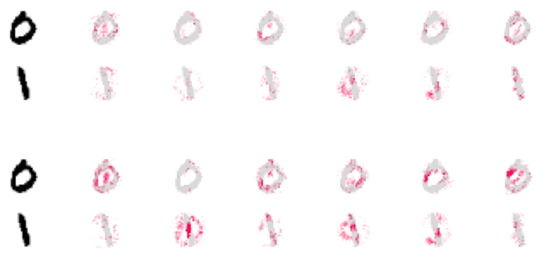
A significant challenge in the current AI landscape arises when neural networks "forget" information they have learned as they are exposed to changing data. Continual Learning (CL) addresses this problem by focusing on training models in dynamic environments where data distributions evolve over time. This scenario is even more challenging when one seeks to explain the predictions of these models, which is a key concern in explainable artificial intelligence (XAI) [1]. In this work, we tackle the problem of explaining models in a CL setting, highlighting how one can represent explanation changes and introducing two novel metrics to assess the effects of non-stationarity in these explanations. The research at the intersection of CL and XAI is extremely limited, with only some attempts to stabilize visual explanations during CL using Replay strategies [2,3]. This study takes a different direction: instead of creating a CL approach that minimizes forgetting, it aims to measure the variation in an explanation and understand how various factors influence it. These factors include the domain of the data, such as images versus sequences, the model architecture, like feedforward (NN) compared to recurrent (RNN) or convolutional (CNN), and the CL strategy used. For this purpose, we investigate the behavior of SHapley Additive exPlanations (SHAP) [4], a popular method in XAI, in a CL classification setting, where new data classes are introduced sequentially. In such a CL scenario, a classifier faces a stream of experiences, i.e., multiple sets of input-target pairs. Each experience introduces a new set of target classes that never reoccur in future experiences. This scenario is well-known to induce a large amount of forgetting in the model. We perform benchmarks on three datasets, split MNIST, CIFAR-10, and SSC [5], and three different models: a feedforward NN, a CNN, and long short-term memory (LSTM) RNN. Further, we compare a Naive strategy to two of the most common CL replay strategies: GSS [6] and Experience Replay (ER). Figure 1 shows an example of the SHAP values saliency maps for each candidate class for the dataset MNIST. In particular, we introduce two classes in each new experience, starting from classes 0 and 1, and the image shows positive SHAP values after training on the last experience (classes 8 and 9). The first column shows the input image, and the other ten columns show the SHAP values for each class (the more active, the higher the pixel's contribution toward the class). Replay (ER) effectively preserves the SHAP values for class 0 and class 1, while Naive is mostly activated by classes 8 and 9 (i.e., the model forgot classes 0 and 1). This means that the model erroneously chooses the last two output units instead of the correct ones (the first two units).

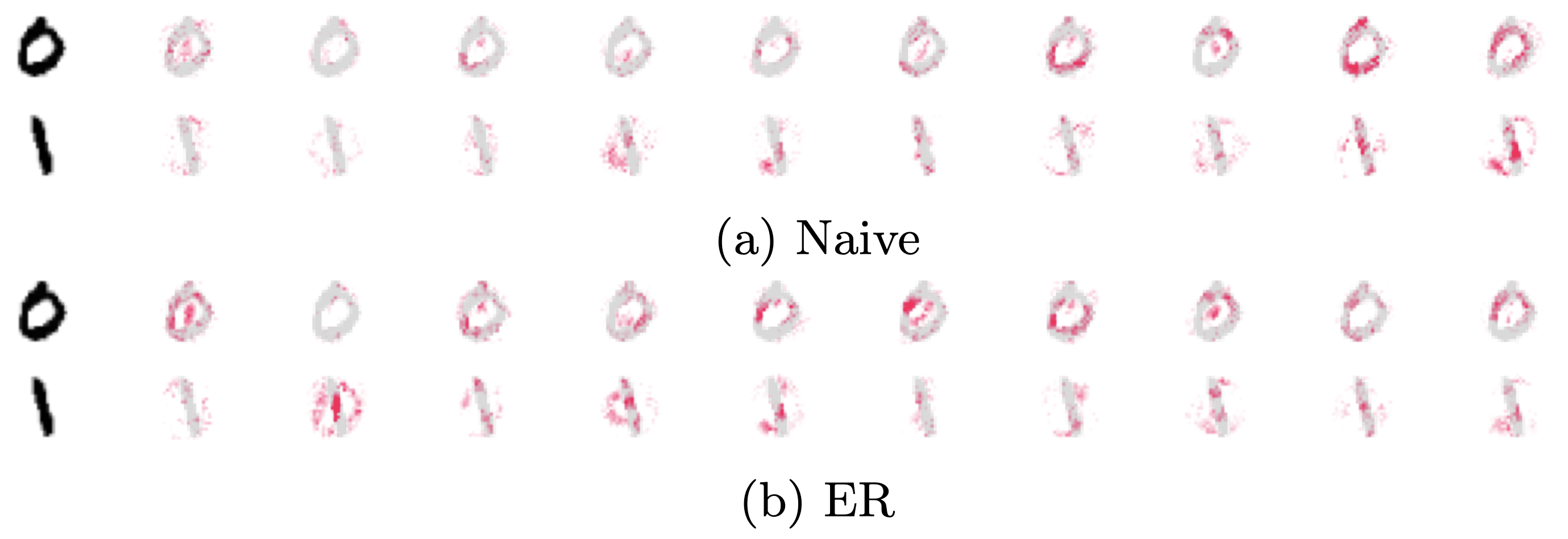
Positive SHAP values after training on the last experience. The first column shows the input image, and the other ten columns show the SHAP values for each class (the more active, the higher the pixel's contribution toward the class). ER is able to effectively preserve the SHAP values for class 0 and class 1, while Naive is mostly activated by class 8 and 9 (forgetting).

In general, we observed that Replay strategies effectively reduce the drift in explanations. However, an exception was observed in RNNs. In these networks, the explanations seemed to drift even more with Replay than when no Continual Learning strategy was applied. We attribute this drift to the recurrent component of RNNs that undergo full training. In fact, when we employed randomized RNNs, the drift in explanation was countered without compromising the model's predictive performance. In conclusion, our study highlights the changes that SHAP undergoes in a CL environment and the unique drift observed in RNN explanations. The research indicates that the fully-trained recurrent component in networks like LSTMs contributes to challenges in maintaining stable explanations. These insights lay the groundwork for future research into ensuring explanation stability in dynamic learning contexts.

References

[1] Riccardo Guidotti, Anna Monreale, Salvatore Ruggieri, Franco Turini, Fosca Giannotti,

and Dino Pedreschi. A survey of methods for explaining black box models. CSUR, 2018.

[2] S. Ebrahimi, S. Petryk, A. Gokul, W. Gan, J. E. Gonzalez, M. Rohrbach, and T. Darrell.

Remembering for the right reasons: Explanations reduce catastrophic forgetting. Applied

AI Letters, 2(4):e44, 2021.

[3] D. Rymarczyk, J. van de Weijer, B. Zielinski, and B. Twardowski. ICICLE: Interpretable

Class Incremental Continual Learning. arxiv, 2023.

[4] Scott M Lundberg and Su-In Lee. A unified approach to interpreting model predictions.

Advances in neural information processing systems, 30, 2017.

[5] A. Cossu, A. Carta, V. Lomonaco, and D. Bacciu. Continual learning for recurrent neural

networks: An empirical evaluation. Neural Networks, 143:607–627, 2021.

[6] R. Aljundi, M. Lin, B. Goujaud, and Y. Bengio. Gradient based sample selection for online

continual learning. In NeurIPS, pages 11816–11825. Curran Associates, Inc., 2019.